Getting started with lsastrat • lsastrat

library(lsastrat)
data(pisa_mini)

What lsastrat does

lsastrat turns large-scale assessment (LSA) data — PISA, TIMSS, PIRLS — into the stratification and inequality quantities that education researchers report, and returns them as first-class objects. It handles the two features that make LSA data awkward:

Plausible values (PVs). Achievement is reported as several imputed draws, not a single score. Every estimator is computed on each PV and the results are combined with Rubin’s (1987) rules, so the measurement uncertainty enters the standard error.
Replicate weights. Complex sampling means the variance must be estimated from replicate weights (BRR/Fay for PISA; JK2 for TIMSS/PIRLS) or, for the segregation indices, a clustered bootstrap.

Inference uses a t reference with Rubin degrees of freedom (not the normal), which matters because LSA studies provide only 5 or 10 plausible values.

What this replaces

Consider the standard workflow for one of the most-reported quantities in educational stratification, the ESCS gradient for a set of countries. Done by hand it means: for each country, fit 10 plausible values x 81 weights = 810 weighted regressions, pool the slopes with Rubin’s rules, derive the strength from the pooled R-squared, and keep track of the Fay factor – then repeat for every country, and again for every robustness variant. General LSA packages (intsvy, EdSurvey, Rrepest) automate the regression but still leave the gradient, segregation indices, opportunity decompositions and their correct inference to be assembled manually, and none applies the finite-sample bias correction the segregation literature calls for. In lsastrat each of these is one call returning a labelled estimate with design-correct uncertainty:

lsa_by(stu, by = "CNT", estimator = social_gradient,
       achievement = paste0("PV", 1:10, "MATH"), escs = "ESCS", design = des)

and tidy() turns any result into a publication table, autoplot() into a figure, and lsa_multiverse() into a robustness analysis.

All examples use pisa_mini, a fully simulated PISA-like data set bundled with the package (it is not real PISA data). It has 10 plausible values each for mathematics and reading (PV1MATH…PV10MATH), a final weight (W_FSTUWT), 64 Fay BRR replicate weights (W_FSTURWT1…W_FSTURWT64), and background variables.

reps <- paste0("W_FSTURWT", 1:64)
math <- paste0("PV", 1:10, "MATH")

The socio-economic gradient

social_gradient() follows the OECD definition: the slope is the score-point change per one unit of the socio-economic index (ESCS), the strength is the percentage of achievement variance it explains (R² × 100), and curvature is an optional quadratic term.

g <- social_gradient(pisa_mini, achievement = math, escs = "ESCS",
                     weight = "W_FSTUWT", repweights = reps)
g
#> Socio-economic achievement gradient
#>   SES index: ESCS   |   10 plausible value(s)   |   n = 2048
#>   Variance:  BRR, 64 replicate weights (+ PV imputation); t reference
#> 
#> 
#>           Estimate Std.Error     t    df       p
#> slope       41.357     1.831 22.59 399.4 2.1e-73
#> strength    20.189     1.799 11.22 389.1 1.7e-25
#> curvature    1.025     1.597  0.64 406.7 5.2e-01
#> 
#> slope = score points per 1 unit of ESCS; strength = % variance explained (R^2 x 100)

The result behaves like a model object:

coef(g)
#>     slope  strength curvature 
#> 41.357302 20.188700  1.025083
confint(g)
#>               2.5 %    97.5 %
#> slope     37.758539 44.956065
#> strength  16.651036 23.726363
#> curvature -2.113944  4.164111

plot(g)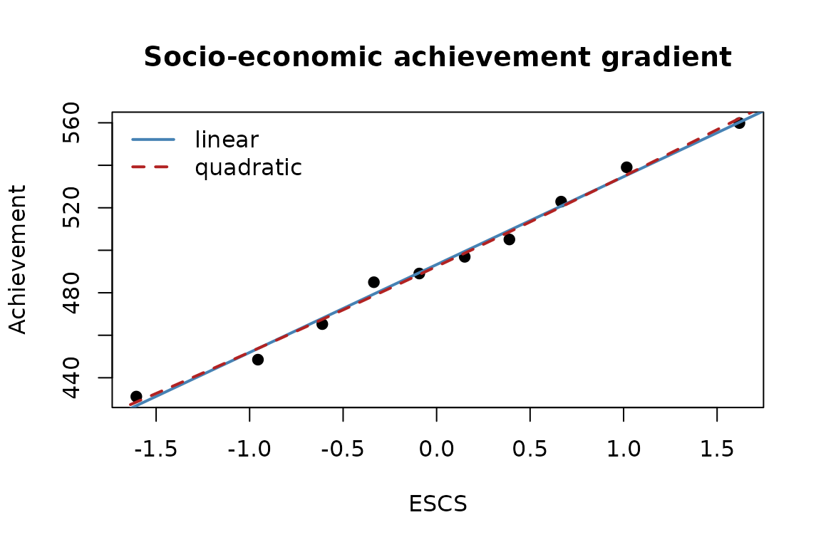

School segregation

segregation_index() reports the family of indices used in stratification research. Pass a categorical group for social segregation:

segregation_index(pisa_mini, unit = "school_id", group = "IMMIG",
                  weight = "W_FSTUWT", variance = "bootstrap",
                  n_boot = 99, boot_seed = 1)
#> Segregation indices (social segregation)
#>   unit: school_id  |  128 units  |  3 group(s)  |  minority: first_gen
#>   Variance: clustered bootstrap (B=99, cluster=school_id), bias-corrected
#> 
#> 
#>           Estimate Std.Error     t  df       p
#> D            0.578     0.037 15.45 Inf 7.8e-54
#> S            0.554     0.040 13.83 Inf 1.7e-43
#> isolation    0.097     0.027  3.55 Inf 3.8e-04
#> Hutchens     0.362     0.036  9.97 Inf 2.2e-23
#> H            0.095     0.017  5.50 Inf 3.9e-08
#> M            0.074     0.016  4.59 Inf 4.3e-06

The entropy and dissimilarity indices are upward-biased when schools are small — exactly the LSA case. With variance = "bootstrap" a two-stage clustered bootstrap estimates and removes that bias (debias = TRUE) and gives a design-correct standard error. With replicate weights you can instead use them directly (no bias correction):

segregation_index(pisa_mini, unit = "school_id", group = "IMMIG",
                  weight = "W_FSTUWT", repweights = reps,
                  indices = c("D", "H", "M"))
#> Segregation indices (social segregation)
#>   unit: school_id  |  128 units  |  3 group(s)  |  minority: first_gen
#>   Variance: BRR, 64 replicate weights; t reference
#> 
#> 
#>   Estimate Std.Error     t  df       p
#> D    0.658     0.040 16.47 Inf 6.2e-61
#> H    0.157     0.012 13.12 Inf 2.5e-39
#> M    0.122     0.011 11.39 Inf 4.8e-30

For academic segregation, define the group by an achievement threshold; the index is then pooled across plausible values:

segregation_index(pisa_mini, unit = "school_id", achievement = math,
                  cutoff = 480, indices = c("D", "H"),
                  variance = "bootstrap", n_boot = 99, boot_seed = 1)
#> No `weight` supplied; using equal weights.
#> Segregation indices (academic segregation)
#>   unit: school_id  |  128 units  |  2 group(s)  |  minority: below
#>   Variance: clustered bootstrap (B=99, cluster=school_id), bias-corrected (+ PV imputation)
#> 
#> 
#>   Estimate Std.Error    t    df       p
#> D    0.218     0.026 8.39 109.0 1.9e-13
#> H    0.052     0.019 2.83 475.3 4.9e-03

Inequality of educational opportunity

ieop() implements the Ferreira–Gignoux (2014) decomposition: the share of achievement variance explained by pre-determined circumstances.

ieop(pisa_mini, achievement = math,
     circumstances = c("IMMIG", "parental_edu", "books"),
     weight = "W_FSTUWT", repweights = reps)
#> Inequality of educational opportunity (Ferreira-Gignoux)
#>   10 plausible value(s)  |  n = 2048  |  3 circumstance(s): IMMIG, parental_edu, books
#>   Variance: BRR, 64 replicate weights (+ PV imputation); t reference
#> 
#> 
#>               Estimate Std.Error     t     df        p
#> iop              0.209     0.018 11.79  612.6  4.6e-29
#> iop_adj          0.206     0.018 11.58  610.7  3.7e-28
#> explained_var 1518.225   143.167 10.60 1204.1  3.5e-25
#> total_var     7253.731   228.176 31.79  517.7 8.7e-124
#> 
#> iop = share of achievement variance explained by circumstances (raw R^2, upper bound); iop_adj = df-adjusted

The raw iop is the regression R² and is an upper bound — it inflates as the circumstance set grows. iop_adj is the degrees-of-freedom adjusted version; prefer it, and treat iop as the ceiling. explained_var is the absolute inequality of opportunity (variance of predicted scores) and total_var the total achievement variance.

Comparing groups

lsa_by() runs any estimator across the levels of a grouping variable and stacks the results into one comparable table – the workhorse for cross-country work. equity_scatter() draws the OECD quality-vs-equity scatter.

by_imm <- lsa_by(pisa_mini, by = "IMMIG", estimator = social_gradient,
                 achievement = math, escs = "ESCS", weight = "W_FSTUWT",
                 repweights = reps)
by_imm
#> `social_gradient` by IMMIG  (3 groups)
#> 
#>       group      term estimate     se statistic       df     p   ci_lo  ci_hi
#>      native     slope   41.867  2.070    20.224  580.355 0.000  37.801 45.933
#>      native  strength   20.192  1.934    10.438  346.181 0.000  16.388 23.997
#>      native curvature    0.752  1.920     0.392  242.884 0.696  -3.031  4.534
#>  second_gen     slope   39.234  3.548    11.058  792.323 0.000  32.269 46.198
#>  second_gen  strength   17.931  2.935     6.108  425.972 0.000  12.161 23.700
#>  second_gen curvature    0.560  2.792     0.201 1125.479 0.841  -4.919  6.039
#>   first_gen     slope   32.697 11.252     2.906  338.768 0.004  10.566 54.829
#>   first_gen  strength   13.126  9.079     1.446  258.647 0.149  -4.752 31.003
#>   first_gen curvature    7.279  8.914     0.817  600.676 0.414 -10.227 24.785

Decomposing inequality

Three decompositions break a quantity into interpretable parts. The between-school variance share (a strongly stratified system has a high value):

variance_decomposition(pisa_mini, math, unit = "school_id",
                       weight = "W_FSTUWT", repweights = reps)
#> Between/within-unit variance decomposition
#>   unit: school_id  |  128 units  |  10 plausible value(s)  |  n = 2048
#>   Variance: BRR, 64 replicate weights (+ PV imputation); t reference
#> 
#> 
#>             Estimate Std.Error     t     df        p
#> icc            0.153     0.017  9.15 1259.2  2.3e-19
#> var_between 1110.411   133.168  8.34 1561.8  1.6e-16
#> var_within  6143.320   205.537 29.89  384.4 2.7e-102
#> var_total   7253.731   228.176 31.79  517.7 8.7e-124
#> 
#> icc = between-unit share of achievement variance

The Shapley decomposition attributes the inequality of opportunity to each circumstance (the contributions sum to the total relative IOp):

ieop_decompose(pisa_mini, math,
               circumstances = c("IMMIG", "parental_edu", "books"),
               weight = "W_FSTUWT", repweights = reps)
#> Inequality of opportunity: Shapley decomposition
#>   10 plausible value(s)  |  n = 2048  |  3 circumstance(s)
#>   Variance: BRR, 64 replicate weights (+ PV imputation); t reference
#> 
#> 
#>              Estimate Std.Error    t    df       p
#> IMMIG           0.009     0.005 2.01 425.3 4.5e-02
#> parental_edu    0.106     0.013 7.86 263.8 9.8e-14
#> books           0.094     0.013 7.44 178.5 4.1e-12
#> 
#> Shapley contributions to relative IOp (R^2); they sum to the total

The Oaxaca-Blinder decomposition splits an achievement gap into an explained (composition) and an unexplained (structure) part:

d2 <- pisa_mini[pisa_mini$IMMIG %in% c("native", "first_gen"), ]
d2$IMMIG <- factor(d2$IMMIG)
oaxaca_gap(d2, math, group = "IMMIG",
           predictors = c("ESCS", "books", "parental_edu"),
           weight = "W_FSTUWT", repweights = reps)
#> Oaxaca-Blinder gap decomposition (twofold)
#>   IMMIG: native - first_gen  |  10 plausible value(s)  |  n = 1421
#>   Variance: BRR, 64 replicate weights (+ PV imputation); t reference
#> 
#> 
#>             Estimate Std.Error    t       df       p
#> gap           32.004     9.690 3.30    627.4 1.0e-03
#> explained     29.250     5.364 5.45 134118.7 5.0e-08
#> unexplained    2.755     8.819 0.31    476.5 7.5e-01
#> 
#> gap = mean(native) - mean(first_gen); components sum to gap

Multiverse analysis

lsa_multiverse() runs an estimator across a grid of analytic forking paths so you can read off how robust a finding is. Bundle the design once with lsa_design():

des <- lsa_design(weight = "W_FSTUWT", repweights = reps)
mv <- lsa_multiverse(
  pisa_mini, estimator = social_gradient,
  grid = list(
    achievement = list(math = math, read = paste0("PV", 1:10, "READ")),
    curvature = list(linear = FALSE, quadratic = TRUE)
  ),
  fixed = list(escs = "ESCS"), design = des, term = "slope")
mv
#> Multiverse: `social_gradient`, term = slope  (4 specifications)
#>   median estimate: 39.1   range: [36.8, 41.4]
#>   100% of specifications same-signed; 100% exclude 0 (95% CI)

Every result has a plot() method, and an autoplot() method when ggplot2 is installed (e.g. autoplot(by_imm, term = "slope") for a forest plot, or autoplot(mv) for the specification curve).

Beyond the built-in estimators

lsa_model() fits any model to a plausible-value outcome with replicate-weight inference – a multiple regression, a logistic model, or a multilevel model – pooling over plausible values exactly as the built-in estimators do. Supply a one-sided formula; the outcome is filled in from each plausible value.

lsa_model(pisa_mini, ~ ESCS + IMMIG + female, achievement = math, design = des)
#> Model: stats::lm(<PV> ~ ESCS + IMMIG + female)
#>   10 plausible value(s)  |  n = 2048
#>   Variance: BRR, 64 replicate weights (+ PV imputation); t reference
#> 
#> 
#>                 Estimate Std.Error      t    df       p
#> (Intercept)      500.857     2.876 174.15 906.1 0.0e+00
#> ESCS              40.659     1.867  21.78 379.4 8.2e-69
#> IMMIGsecond_gen   -9.437     4.284  -2.20 223.0 2.9e-02
#> IMMIGfirst_gen    -3.537     9.344  -0.38 470.4 7.1e-01
#> female            -9.770     4.599  -2.12 279.3 3.5e-02
#> 
#> fitter = stats::lm

lsa_trend() compares a quantity across assessment cycles and folds the linking (equating) error into the standard error of the change:

half <- nrow(pisa_mini) %/% 2
c1 <- social_gradient(pisa_mini[1:half, ], math, "ESCS", design = des)
c2 <- social_gradient(pisa_mini[-(1:half), ], math, "ESCS", design = des)
lsa_trend(list("2018" = c1, "2022" = c2), term = "slope", link_error = 3.5)
#> Trend in `slope` (social_gradient) across 2 cycles; baseline = 2018
#>   linking error: 3.5 (added to each change SE)
#> 
#>  cycle estimate    se change change.se    z    p
#>   2018   41.308 2.874  0.000        NA   NA   NA
#>   2022   41.454 2.426  0.146     5.137 0.03 0.98
#> 
#> change = estimate - baseline; SE includes the linking error

On large data the replicate-weight refits can be run in parallel with options(lsastrat.cores = 4) (Unix/macOS).

Where it fits

lsastrat complements rather than replaces general LSA packages such as EdSurvey, intsvy, BIFIEsurvey, RALSA and OECD’s Rrepest, which provide the generic estimators but leave these stratification quantities to be assembled by hand. The estimators are cross-validated against intsvy::pisa.reg.pv(), the segregation package, and a weighted regression R². ```